ds-algo-study

# Recursion Practice --- --- ### TODO: >Implement with jsfiddle so people can see the specs and their code in the same window rather than a combo of editor/browser --- ### **How to use this repo:** 1. Fork this repo and clone it to your local machine 2. Open `SpecRunner.html` in your web browser 3. Code your solutions in `recursion.js` 4. Review the tests in `spec/part1.js` and `spec/part2.js` as necessary 5. Save your work and refresh your browser to check for passing/failing tests --- ### What is recursion? > Recursion is when a function calls itself until it doesn't. --not helpful person Is it a true definition? Mostly. Recursion is when a function calls itself. A recursive function can call itself forever, but that's generally not preferred. It's often a good idea to include a condition in the function definition that allows it to stop calling itself. This condition is referred to as a **_base_** case. As a general rule, recursion shouldn't be utilized without an accompanying base case unless an infinite operation is desired. This leaves us with two fundamental conditions every recursive function should include: - A **`base`** case - A **`recursive`** case _What does this all mean?_ Let's consider a silly example: ```javascript function stepsToZero(n) { if (n === 0) { /* base case */ return 'Reached zero'; } else { /* recursive case */ console.log(n + ' is not zero'); return stepsToZero(n-1); } } ``` This function doesn't do anything meaningful, but hopefully it demonstrates the fundamental idea behind recursion. Simply put, recursion provides us a looping or repeating mechanism. It repeats an operation until a `base` condition is met. Let's step through an invocation of the above function to see how it evaluates. 1. Invoke `stepsToZero(n)` where `n` is the number `2` 2. Is 2 zero? 3. No, print message to console that 2 is not zero 4. Invoke `stepsToZero(n-1)` where `n-1` evaluates to `1` > Every recursive call adds a new invocation to the stack on top of the previous invocation 5. Is 1 zero? 6. No, print message that 1 is not zero 7. Invoke `stepsToZero(n-1)` where `n-1` evaluates to `0` 8. Is 0 zero? 9. Yes, return message that reached zero 10. The above return pops the current invocation off the stack 6. Resume the invocation from step 4 where it left off (in-between steps 6 and 7) 6. Return out of the invocation from step 4 12. Resume the initial invocation from step 1 where it left off (in-between steps 3 and 4) 12. Return out of the initial invocation Note that the value returned from the base case (step 9) gets returned to the previous invocation (step 4) on the stack. Step 4's invocation takes that value and returns it to the invocation that preceded it (step 1). Once the initial invocation is reached, it returns the value to whatever invoked it. Through these steps, you can watch the call stack build up and once the base case is reached, the return value is passed back down as each invocation pops off the stack. Due to the way the execution stack operates, it's as if each function invocation pauses in time when a recursive call is made. The function that pauses before a recursive call will resume once the recursive call completes. If you've seen the movie [Inception], this model may sound reminiscent to when the characters enter a person's dreams and time slowed. The difference is time doesn't actually slow with recursive invocations; rather, it's a matter of order of operations. If a new invocation enters the execution stack, that invocation must complete before the previous can continue and complete. ### Why use recursion? Recursion can be elegant, but it can also be dangerous. In some cases, recursion feels like a more natural and readable solution; in others, it ends up being contrived. In most cases, recursion can be avoided entirely and sometimes should in order to minimize the possibility of exceeding the call stack and crashing your app. But keep in mind that code readability is important. If a recursive solution reads more naturally, then it may be the best solution for the given problem. Recursion isn't unique to any one programming language. As a software engineer, you _will_ encounter recursion and it's important to understand what's happening and how to work with it. It's also important to understand why someone might use it. Recursion is often used when the depth of a thing is unknown or every element of a thing needs to be touched. For example, you might use recursion if you want to find all DOM elements with a specific class name. You may not know how deep the DOM goes and need to touch every element so that none are missed. The same can be said for traversing any structure where all possible paths need to be considered and investigated. ### Divide and Conquer Recursion is often used in _divide and conquer_ algorithms where problems can be divided into similar subproblems and conquered individually. Consider traversing a tree structure. Each branch may have its own "children" branches. Every branch is essentially just another tree which means, as long as child trees are found, we can recurse on each child. [inception]: <https://en.wikipedia.org/wiki/Inception> > What's the difference and connections between recursion, divide-and-conquer algorithm, dynamic programming, and greedy algorithm? If you haven't made it clear. Doesn't matter! I would give you a brief introduction to kick off this section. What's the difference and connections between recursion, divide-and-conquer algorithm, dynamic programming, and greedy algorithm? If you haven't made it clear. Doesn't matter! I would give you a brief introduction to kick off this section. Recursion is a programming technique. It's a way of thinking about solving problems. There're two algorithmic ideas to solve specific problems: divide-and-conquer algorithm and dynamic programming. They're largely based on recursive thinking (although the final version of dynamic programming is rarely recursive, the problem-solving idea is still inseparable from recursion). There's also an algorithmic idea called greedy algorithm which can efficiently solve some more special problems. And it's a subset of dynamic programming algorithms. The divide-and-conquer algorithm will be explained in this section. Taking the most classic merge sort as an example, it continuously divides the unsorted array into smaller sub-problems. This is the origin of the word **divide and conquer**. Obviously, the sub-problems decomposed by the ranking problem are non-repeating. If some of the sub-problems after decomposition are duplicated (the nature of overlapping sub-problems), then the dynamic programming algorithm is used to solve them! ``` . ├── AUX_MATERIALS │ ├── recursion-flow.PNG │ ├── right.html │ ├── sandbox │ │ ├── LOs.js │ │ ├── example2.js │ │ ├── examples.js │ │ ├── exponent.js │ │ ├── factorial.js │ │ ├── fibonacci.js │ │ ├── flatten.js │ │ ├── memoize.js │ │ ├── recursiveCallStack.js │ │ ├── recursiveIsEven.js │ │ ├── recursiveRange.js │ │ ├── right.html │ │ ├── sum.js │ │ └── tabulate.js │ ├── solved.pdf │ └── unzolved.pdf ├── README.html ├── README.md ├── blank │ ├── README.md │ ├── SpecRunner.html │ ├── lib │ │ ├── chai.js │ │ ├── css │ │ │ ├── mocha.css │ │ │ └── right.html │ │ ├── jquery.js │ │ ├── mocha.js │ │ ├── right.html │ │ ├── sinon.js │ │ └── testSupport.js │ ├── right.html │ ├── spec │ │ ├── part1.js │ │ ├── part2.js │ │ └── right.html │ ├── src │ │ ├── recursion.js │ │ └── right.html │ └── testing │ ├── directory1.html │ ├── left1.html │ ├── prism.css │ ├── prism.js │ ├── right.html │ ├── right1.html │ └── starter.html ├── dir.md ├── directory.html ├── images │ ├── BubbleSort.gif │ ├── InsertionSort.gif │ ├── MergeSort.gif │ ├── QuickSort.gif │ ├── SLL-diagram.png │ ├── SelectionSort.gif │ ├── array-in-memory.png │ ├── fib_memoized.png │ ├── fib_tree.png │ ├── fib_tree_duplicates.png │ ├── github-repo-menu-bar-wiki.png │ └── right.html ├── index.html ├── left.html ├── my-solutions │ ├── README.md │ ├── SpecRunner.html │ ├── complete.html │ ├── lib │ │ ├── chai.js │ │ ├── css │ │ │ ├── mocha.css │ │ │ └── right.html │ │ ├── jquery.js │ │ ├── mocha.js │ │ ├── right.html │ │ ├── sinon.js │ │ └── testSupport.js │ ├── prism.css │ ├── prism.js │ ├── right.html │ ├── spec │ │ ├── part1.js │ │ ├── part2.js │ │ └── right.html │ ├── src │ │ ├── recursion.js │ │ └── right.html │ └── style.css ├── part-2 │ ├── README.md │ ├── SpecRunner.html │ ├── lib │ │ ├── jasmine-1.0.0 │ │ │ ├── MIT.LICENSE │ │ │ ├── jasmine-html.js │ │ │ ├── jasmine.css │ │ │ ├── jasmine.js │ │ │ └── right.html │ │ ├── right.html │ │ └── underscore.js │ ├── right.html │ ├── solutions │ │ ├── binarySearchTree.js │ │ ├── hashTable.js │ │ ├── hashTableHelpers.js │ │ ├── linkedList.js │ │ ├── right.html │ │ ├── set.js │ │ └── tree.js │ ├── spec │ │ ├── binarySearchTreeSpec.js │ │ ├── hashTableSpec.js │ │ ├── linkedListSpec.js │ │ ├── right.html │ │ ├── setSpec.js │ │ └── treeSpec.js │ └── src │ ├── binarySearchTree.js │ ├── hashTable.js │ ├── hashTableHelpers.js │ ├── linkedList.js │ ├── right.html │ ├── set.js │ └── tree.js ├── prism.css ├── prism.js ├── right.html ├── style.css ├── tabs │ ├── right.html │ ├── tabs.html │ ├── tabs2.html │ └── template-files │ ├── LmfE5ZMlM8QjZWyylbaJdeYzodpJKK3mlCt6sCr3jaw.js │ ├── about-us-page-template.jpg │ ├── ad_status.js │ ├── agency-template.jpg │ ├── analytics.js │ ├── application-template.jpg │ ├── article-template.jpg │ ├── base.js │ ├── best-bootstrap-templates-492x492.jpg │ ├── blog.jpg │ ├── bootstrap-basic-template-492x492.jpg │ ├── bootstrap-ecommerce-template-492x492.jpg │ ├── bootstrap-grid.min.css │ ├── bootstrap-landing-page-template-492x492.jpg │ ├── bootstrap-layout-templates-492x492.jpg │ ├── bootstrap-login-page-template-492x492.jpg │ ├── bootstrap-one-page-template-492x492.jpg │ ├── bootstrap-page-templates-492x492.jpg │ ├── bootstrap-portfolio-template-600x600.jpg │ ├── bootstrap-reboot.min.css │ ├── bootstrap-responsive-website-templates-600x600.jpg │ ├── bootstrap-sample-template-492x492.jpg │ ├── bootstrap-single-page-template-492x492.jpg │ ├── bootstrap-starter-template-492x492.jpg │ ├── bootstrap-templates-examples-492x492.jpg │ ├── bootstrap-theme-template-492x492.jpg │ ├── bootstrap.min.css │ ├── bootstrap.min.js │ ├── business-template.jpg │ ├── carousel-template.jpg │ ├── cast_sender.js │ ├── coming-soon-template.jpg │ ├── contact-form-template-1.jpg │ ├── corporate-template.jpg │ ├── documentation-template.jpg │ ├── download-bootstrap-template-492x492.jpg │ ├── education-template.jpg │ ├── embed.js │ ├── error-template.jpg │ ├── event-template.jpg │ ├── f(1).txt │ ├── f.txt │ ├── faq-template.jpg │ ├── fbevents.js │ ├── fetch-polyfill.js │ ├── footer-template.jpg │ ├── form-templates.jpg │ ├── free-html5-bootstrap-templates-600x600.jpg │ ├── gallery-template.jpg │ ├── google-maps-template.jpg │ ├── grid-template.jpg │ ├── gtm.js │ ├── hGaQaBeUfGw.html │ ├── header-template.jpg │ ├── homepage-template.jpg │ ├── hotel-template.jpg │ ├── jarallax.min.js │ ├── jquery.min.js │ ├── jquery.touch-swipe.min.js │ ├── landing-page-template.jpg │ ├── list-template.jpg │ ├── magazine-template.jpg │ ├── map-template.jpg │ ├── mbr-additional.css │ ├── menu-template.jpg │ ├── mobirise-icons.css │ ├── multi-page-template.jpg │ ├── navbar-template.jpg │ ├── navigation-menu.jpg │ ├── news-template.jpg │ ├── one-page-1.jpg │ ├── ootstrap-design-template-492x492.jpg │ ├── parallax-scrolling-template.jpg │ ├── parallax-template.jpg │ ├── personal-website-template.jpg │ ├── photo-gallery-template.jpg │ ├── photography-template.jpg │ ├── popper.min.js │ ├── premium-bootstrap-templates-492x492.jpg │ ├── profile-template.jpg │ ├── real-estate-template.jpg │ ├── registration-form-template.jpg │ ├── remote.js │ ├── restaurant-template.jpg │ ├── right.html │ ├── script.js │ ├── script.min.js │ ├── shopping-cart.jpg │ ├── simple-bootstrap-template-492x492.jpg │ ├── slider-template.jpg │ ├── slider.jpg │ ├── smooth-scroll.js │ ├── social-network-template.jpg │ ├── store-template.jpg │ ├── style(1).css │ ├── style.css │ ├── tab-template.jpg │ ├── table-template.jpg │ ├── tether.min.css │ ├── tether.min.js │ ├── travel-template.jpg │ ├── video-bg-template.jpg │ ├── video-bg.jpg │ ├── video-gallery-template.jpg │ ├── video-template.jpg │ ├── warren-wong-200912-2000x1304.jpg │ ├── web-application-template.jpg │ ├── wedding-template.jpg │ ├── www-embed-player.js │ └── www-player-webp.css └── tree.md 22 directories, 227 files ``` Recursion in detail ------------------- Before introducing divide and conquer algorithm, we must first understand the concept of recursion. The basic idea of recursion is that a function calls itself directly or indirectly, which transforms the solution of the original problem into many smaller sub-problems of the same nature. All we need is to focus on how to divide the original problem into qualified sub-problems, rather than study how this sub-problem is solved. The difference between recursion and enumeration is that enumeration divides the problem horizontally and then solves the sub-problems one by one, but recursion divides the problem vertically and then solves the sub-problems hierarchily. The following illustrates my understanding of recursion. **If you don't want to read, please just remember how to answer these questions:** 1. How to sort a bunch of numbers? Answer: Divided into two halves, first align the left half, then the right half, and finally merge. As for how to arrange the left and right half, please read this sentence again. 2. How many hairs does Monkey King have? Answer: One plus the rest. 3. How old are you this year? Answer: One year plus my age of last year, I was born in 1999. Two of the most important characteristics of recursive code: **end conditions and self-invocation**. Self-invocation is aimed at solving sub-problems, and the end condition defines the answer to the simplest sub-problem. Actually think about it, **what is the most successful application of recursion? I think it's mathematical induction**. Most of us learned mathematical induction in high school. The usage scenario is probably: we can't figure out a summation formula, but we tried a few small numbers which seemed containing a kinda law, and then we compiled a formula. We ourselves think it shall be the correct answer. However, mathematics is very rigorous. Even if you've tried 10,000 cases which are correct, can you guarantee the 10001th correct? This requires mathematical induction to exert its power. Assuming that the formula we compiled is true at the kth number, furthermore if it is proved correct at the k + 1th, then the formula we have compiled is verified correct. So what is the connection between mathematical induction and recursion? We just said that the recursive code must have an end condition. If not, it will fall into endless self-calling hell until the memory exhausted. The difficulty of mathematical proof is that you can try to have a finite number of cases, but it is difficult to extend your conclusion to infinity. Here you can see the connection-infinite. The essence of recursive code is to call itself to solve smaller sub-problems until the end condition is reached. The reason why mathematical induction is useful is to continuously increase our guess by one, and expand the size of the conclusion, without end condition. So by extending the conclusion to infinity, the proof of the correctness of the guess is completed. ### Why learn recursion First to train the ability to think reversely. Recursive thinking is the thinking of normal people, always looking at the problems in front of them and thinking about solutions, and the solution is the future tense; Recursive thinking forces us to think reversely, see the end of the problem, and treat the problem-solving process as the past tense. Second, practice analyzing the structure of the problem. When the problem can be broken down into sub problems of the same structure, you can acutely find this feature, and then solve it efficiently. Third, go beyond the details and look at the problem as a whole. Let's talk about merge and sort. In fact, you can divide the left and right areas without recursion, but the cost is that the code is extremely difficult to understand. Take a look at the code below (merge sorting will be described later. You can understand the meaning here, and appreciate the beauty of recursion). void sort(Comparable[] a){ int N = a.length; // So complicated! It shows disrespect for sorting. I refuse to study such code. for (int sz = 1; sz < N; sz = sz + sz) for (int lo = 0; lo < N - sz; lo += sz + sz) merge(a, lo, lo + sz - 1, Math.min(lo + sz + sz - 1, N - 1)); } /* I prefer recursion, simple and beautiful */ void sort(Comparable[] a, int lo, int hi) { if (lo >= hi) return; int mid = lo + (hi - lo) / 2; sort(a, lo, mid); // soft left part sort(a, mid + 1, hi); // soft right part merge(a, lo, mid, hi); // merge the two sides } Looks simple and beautiful is one aspect, the key is **very interpretable**: sort the left half, sort the right half, and finally merge the two sides. The non-recursive version looks unintelligible, full of various incomprehensible boundary calculation details, is particularly prone to bugs and difficult to debug. Life is short, i prefer the recursive version. Obviously, sometimes recursive processing is efficient, such as merge sort, **sometimes inefficient**, such as counting the hair of Monkey King, because the stack consumes extra space but simple inference does not consume space. Example below gives a linked list header and calculate its length: ### Tips for writing recursion My point of view: **Understand what a function does and believe it can accomplish this task. Don't try to jump into the details.** Do not jump into this function to try to explore more details, otherwise you will fall into infinite details and cannot extricate yourself. The human brain carries tiny sized stack! Let's start with the simplest example: traversing a binary tree. Above few lines of code are enough to wipe out any binary tree. What I want to say is that for the recursive function `traverse (root)` , we just need to believe: give it a root node `root` , and it can traverse the whole tree. Since this function is written for this specific purpose, so we just need to dump the left and right nodes of this node to this function, because I believe it can surely complete the task. What about traversing an N-fork tree? It's too simple, exactly the same as a binary tree! As for pre-order, mid-order, post-order traversal, they are all obvious. For N-fork tree, there is obviously no in-order traversal. The following **explains a problem from LeetCode in detail**: Given a binary tree and a target value, the values in every node is positive or negative, return the number of paths in the tree that are equal to the target value, let you write the pathSum function: The problem may seem complicated, but the code is extremely concise, which is the charm of recursion. Let me briefly summarize the **solution process** of this problem: First of all, it is clear that to solve the problem of recursive tree, you must traverse the entire tree. So the traversal framework of the binary tree (recursively calling the function itself on the left and right children) must appear in the main function pathSum. And then, what should they do for each node? They should see how many eligible paths they and their little children have under their feet. Well, this question is clear. According to the techniques mentioned earlier, define what each recursive function should do based on the analysis just now: PathSum function: Give it a node and a target value. It returns the total number of paths in the tree rooted at this node and the target value. Count function: Give it a node and a target value. It returns a tree rooted at this node, and can make up the total number of paths starting with the node and the target value. /* With above tips, comment out the code in detail */ int pathSum(TreeNode root, int sum) { if (root == null) return 0; int pathImLeading = count(root, sum); // Number of paths beginning with itself int leftPathSum = pathSum(root.left, sum); // The total number of paths on the left (Believe he can figure it out) int rightPathSum = pathSum(root.right, sum); // The total number of paths on the right (Believe he can figure it out) return leftPathSum + rightPathSum + pathImLeading; } int count(TreeNode node, int sum) { if (node == null) return 0; // Can I stand on my own as a separate path? int isMe = (node.val == sum) ? 1 : 0; // Left brother, how many sum-node.val can you put together? int leftBrother = count(node.left, sum - node.val); // Right brother, how many sum-node.val can you put together? int rightBrother = count(node.right, sum - node.val); return isMe + leftBrother + rightBrother; // all count i can make up } Again, understand what each function can do and trust that they can do it. In summary, the binary tree traversal framework provided by the PathSum function calls the count function for each node during the traversal. Can you see the pre-order traversal (the order is the same for this question)? The count function is also a binary tree traversal, used to find the target value path starting with this node. Understand it deeply! Divide and conquer algorithm ---------------------------- **Merge and sort**, typical divide-and-conquer algorithm; divide-and-conquer, typical recursive structure. The divide-and-conquer algorithm can go in three steps: decomposition-> solve-> merge 1. Decompose the original problem into sub-problems with the same structure. 2. After decomposing to an easy-to-solve boundary, perform a recursive solution. 3. Combine the solutions of the subproblems into the solutions of the original problem. To merge and sort, let's call this function `merge_sort` . According to what we said above, we must clarify the responsibility of the function, that is, **sort an incoming array**. OK, can this problem be solved? Of course! Sorting an array is just the same to sorting the two halves of the array separately, and then merging the two halves. Well, this algorithm is like this, there is no difficulty at all. Remember what I said before, believe in the function's ability, and pass it to him half of the array, then the half of the array is already sorted. Have you found it's a binary tree traversal template? Why it is postorder traversal? Because the routine of our divide-and-conquer algorithm is **decomposition-> solve (bottom)-> merge (backtracking)** Ah, first left and right decomposition, and then processing merge, backtracking is popping stack, which is equivalent to post-order traversal. As for the `merge` function, referring to the merging of two ordered linked lists, they are exactly the same, and the code is directly posted below. Let's refer to the Java code in book `Algorithm 4` below, which is pretty. This shows that not only algorithmic thinking is important, but coding skills are also very important! Think more and imitate more. ```java public class Merge { // Do not construct new arrays in the merge function, because the merge function will be called multiple times, affecting performance.Construct a large enough array directly at once, concise and efficient. private static Comparable[] aux; public static void sort(Comparable[] a) { aux = new Comparable[a.length]; sort(a, 0, a.length - 1); } private static void sort(Comparable[] a, int lo, int hi) { if (lo >= hi) return; int mid = lo + (hi - lo) / 2; sort(a, lo, mid); sort(a, mid + 1, hi); merge(a, lo, mid, hi); } private static void merge(Comparable[] a, int lo, int mid, int hi) { int i = lo, j = mid + 1; for (int k = lo; k <= hi; k++) aux[k] = a[k]; for (int k = lo; k <= hi; k++) { if (i > mid) { a[k] = aux[j++]; } else if (j > hi) { a[k] = aux[i++]; } else if (less(aux[j], aux[i])) { a[k] = aux[j++]; } else { a[k] = aux[i++]; } } } private static boolean less(Comparable v, Comparable w) { return v.compareTo(w) < 0; } } ``` LeetCode has a special exercise of the divide-and-conquer algorithm. Copy the link below to web browser and have a try: https://leetcode.com/tag/divide-and-conquer/ Prompt: write a function that will reverse a string: var reverse = function(string){ if(string.length < 2){ } var first = string\[0\] var last = string\[string.length-1\]; return last +reverse(string.slice(1, string.length-1)) + first; }; reverse('abcdef'); //returns 'fedcba' **//explain what a recursive function is** **_A function that calls itself_** is a recursive function. If a function calls itself… then that function calls itself… then that function calls itself… well… then we have fallen into an infinite loop (a very unproductive place to be). To benefit from recursive calls, we need to be careful to include to give our interpreter a way to break out of the cycle of recursive function calls; we call this a **_base case_**. The base case in the solution code above is as simple as testing that the length of the argument is less than 2… and if it is, returning the the value of that argument. Notice how each time we recursively call the reverse function, we are passing it a shorter string argument… so each recursive call is getting us closer to hitting our **_base case_**. 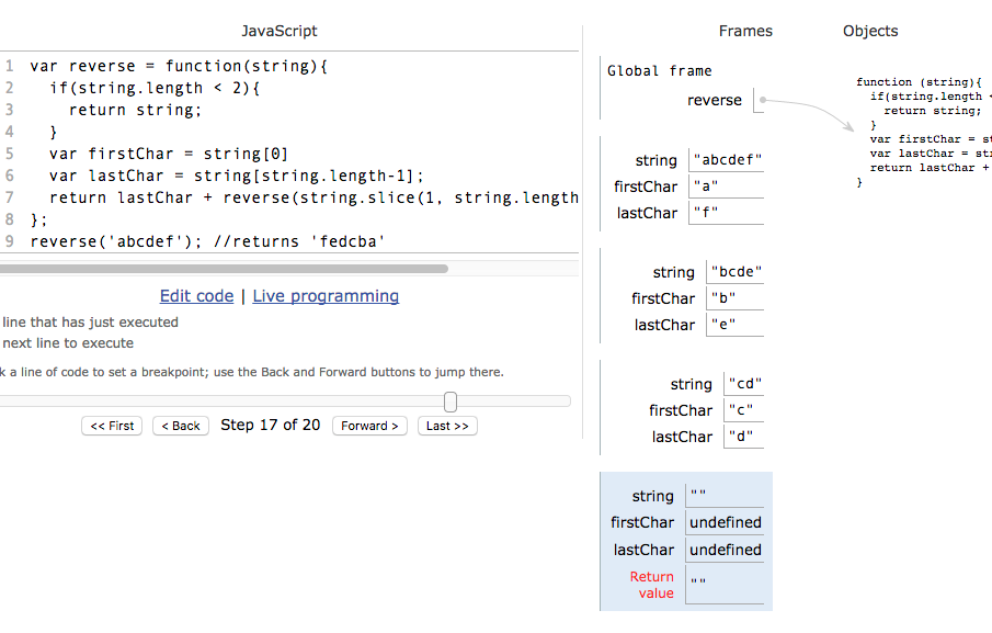**//visualize the interpreter's path through recursive function calls** ![Image for post](https://miro.medium.com/max/60/1*J4FL6LpLY1AXy_KPFdREKw.png?q=20) Image for post ![Image for post](https://miro.medium.com/max/1810/1*J4FL6LpLY1AXy_KPFdREKw.png) Image for post Slow down and follow the interpreter through its execution of your algorithm (thanks to PythonTutor.com) Python Tutor is an excellent resource for learning to visualize and trace variable values through the multiple execution contexts of a recursive function's invocation. _Try it now with these simple steps:_ 1. _copy the solution code from above_ 2. _go over to_ [_http://pythontutor.com/javascript.html#mode=edit_](http://pythontutor.com/javascript.html#mode=edit) 3. _paste the solution code into the editor_ 4. _click the "Visualize Execution" button_ 5. _progress through the execution with the "forward" button_ **//when can a recursive function help me?** So if I hope that at this point that you are thinking: there is a **_better_** way to reverse a function, or there is a **_simpler_** way to reverse a string… First off… **_simpler is better._** Writing good code isn't about being clever or fancy; good code is about writing code that works, that makes sense to as many other minds as possible, that is time efficient, and that is memory efficient (in order of importance). As new programers, the first of these criteria is obvious, and the last two are given way too much weight. It's the second of these criteria that needs to carry much more weight in our minds and deserves the most attention. Recursive functions can be a powerful tool in helping us write clear and simple solutions. To be clear: recursion is not about being fancy or clever… it is an important skill to wrestle with early because there will be many scenarios when employing recursion will allow for a simpler and more reliable solution than would be possible without recursive functions. **//more useful example** Prompt: check to see if a binary-search-tree contains a value ```js var searchBST = function(tree, num){ if(tree.val === num){ } else if(num > tree.val){ } else{ } }; var tree = {val: 9, searchBST(tree, 4) // return false ``` When traversing trees and many other other non-primative data structures, recursion allows us to define a clear algorithm that elegantly handles uncertainty and complexity. Without recursion, it would be impossible to write a single function that could search a binary search tree of any size and state… yet by employing recursion, we can write a concise algorithm that will traverse any binary search tree and determine if it contains a value or not. Take a moment to analyze how recursion is used in this example by tracing the interpreters path through this solution. Just as we did for the reverse function above, paste this binary search tree code snippet into the editor at [http://pythontutor.com/javascript.html#mode=display](http://pythontutor.com/javascript.html#mode=display) In this function definition, there are three base cases that will return a value instead of recursively calling the searchBST function… can you find them? //now go practice using recursion --- * * * [**Big O**](#big-o-) [**Memoization And Tabulation**](#memoization-and-tabulation-) \- [Recursion Videos](#recursion-videos) - [Curating Complexity: A Guide to Big-O Notation](#curating-complexity-a-guide-to-big-o-notation) - [Why Big-O?](#why-big-o) - [Big-O Notation](#big-o-notation) - [Common Complexity Classes](#common-complexity-classes) - [The seven major classes](#the-seven-major-classes) - [Memoization](#memoization) - [Memoizing factorial](#memoizing-factorial) - [Memoizing the Fibonacci generator](#memoizing-the-fibonacci-generator) - [The memoization formula](#the-memoization-formula) - [Tabulation](#tabulation) - [Tabulating the Fibonacci number](#tabulating-the-fibonacci-number) - [Aside: Refactoring for O(1) Space](#aside-refactoring-for-o1-space) - [Analysis of Linear Search](#analysis-of-linear-search) - [Analysis of Binary Search](#analysis-of-binary-search) - [Analysis of the Merge Sort](#analysis-of-the-merge-sort) - [Analysis of Bubble Sort](#analysis-of-bubble-sort) - [LeetCode.com](#leetcodecom) - [Memoization Problems](#memoization-problems) - [Tabulation Problems](#tabulation-problems) [**Sorting Algorithms**](#sorting-algorithms-) \- [Bubble Sort](#bubble-sort) - [_"But…then…why are we…"_](#_butthenwhy-are-we_) - [The algorithm bubbles up](#the-algorithm-bubbles-up) - [How does a pass of Bubble Sort work?](#how-does-a-pass-of-bubble-sort-work) - [Ending the Bubble Sort](#ending-the-bubble-sort) - [Pseudocode for Bubble Sort](#pseudocode-for-bubble-sort) - [Selection Sort](#selection-sort) - [The algorithm: select the next smallest](#the-algorithm-select-the-next-smallest) - [The pseudocode](#the-pseudocode) - [Insertion Sort](#insertion-sort) - [The algorithm: insert into the sorted region](#the-algorithm-insert-into-the-sorted-region) - [The Steps](#the-steps) - [The pseudocode](#the-pseudocode-1) - [Merge Sort](#merge-sort) - [The algorithm: divide and conquer](#the-algorithm-divide-and-conquer) - [Quick Sort](#quick-sort) - [How does it work?](#how-does-it-work) - [The algorithm: divide and conquer](#the-algorithm-divide-and-conquer-1) - [The pseudocode](#the-pseudocode-2) - [Binary Search](#binary-search) - [The Algorithm: "check the middle and half the search space"](#the-algorithm-check-the-middle-and-half-the-search-space) - [The pseudocode](#the-pseudocode-3) - [Bubble Sort Analysis](#bubble-sort-analysis) - [Time Complexity: O(n2)](#time-complexity-onsup2sup) - [Space Complexity: O(1)](#space-complexity-o1) - [When should you use Bubble Sort?](#when-should-you-use-bubble-sort) - [Selection Sort Analysis](#selection-sort-analysis) - [Selection Sort JS Implementation](#selection-sort-js-implementation) - [Time Complexity Analysis](#time-complexity-analysis) - [Space Complexity Analysis: O(1)](#space-complexity-analysis-o1) - [When should we use Selection Sort?](#when-should-we-use-selection-sort) - [Insertion Sort Analysis](#insertion-sort-analysis) - [Time and Space Complexity Analysis](#time-and-space-complexity-analysis) - [When should you use Insertion Sort?](#when-should-you-use-insertion-sort) - [Merge Sort Analysis](#merge-sort-analysis) - [Full code](#full-code) - [Merging two sorted arrays](#merging-two-sorted-arrays) - [Divide and conquer, step-by-step](#divide-and-conquer-step-by-step) - [Time and Space Complexity Analysis](#time-and-space-complexity-analysis-1) - [Quick Sort Analysis](#quick-sort-analysis) - [Time and Space Complexity Analysis](#time-and-space-complexity-analysis-2) - [Binary Search Analysis](#binary-search-analysis) - [Time and Space Complexity Analysis](#time-and-space-complexity-analysis-3) - [Practice: Bubble Sort](#practice-bubble-sort) - [Practice: Selection Sort](#practice-selection-sort) - [Practice: Insertion Sort](#practice-insertion-sort) - [Practice: Merge Sort](#practice-merge-sort) - [Practice: Quick Sort](#practice-quick-sort-2) - [Practice: Binary Search](#practice-binary-search) [**Lists, Stacks, and Queues**](#lists-stacks-and-queues-) \- [Linked Lists](#linked-lists) - [What is a Linked List?](#what-is-a-linked-list) - [Types of Linked Lists](#types-of-linked-lists) - [Linked List Methods](#linked-list-methods) - [Time and Space Complexity Analysis](#time-and-space-complexity-analysis-4) - [Time Complexity - Access and Search](#time-complexity-access-and-search) - [Time Complexity - Insertion and Deletion](#time-complexity-insertion-and-deletion) - [Space Complexity](#space-complexity-1) - [Stacks and Queues](#stacks-and-queues) - [What is a Stack?](#what-is-a-stack) - [What is a Queue?](#what-is-a-queue) - [Stack and Queue Properties](#stack-and-queue-properties) - [Stack Methods](#stack-methods) - [Queue Methods](#queue-methods) - [Time and Space Complexity Analysis](#time-and-space-complexity-analysis-5) - [When should we use Stacks and Queues?](#when-should-we-use-stacks-and-queues) - [**Graphs and Heaps**](#graphs-and-heaps-) \- [Introduction to Heaps](#introduction-to-heaps) - [Binary Heap Implementation](#binary-heap-implementation) - [Heap Sort](#heap-sort) - [In-Place Heap Sort](#in-place-heap-sort) - * * * **The objective of this lesson** is get you comfortable with identifying the time and space complexity of code you see. Being able to diagnose time complexity for algorithms is an essential for interviewing software engineers. At the end of this, you will be able to 1. Order the common complexity classes according to their growth rate 2. Identify the complexity classes of common sort methods 3. Identify complexity classes of codeable with identifying the time and space complexity of code you see. Being able to diagnose time complexity for algorithms is an essential for interviewing software engineers. At the end of this, you will be able to 1. Order the common complexity classes according to their growth rate 2. Identify the complexity classes of common sort methods 3. Identify complexity classes of code * * * **The objective of this lesson** is to give you a couple of ways to optimize a computation (algorithm) from a higher complexity class to a lower complexity class. Being able to optimize algorithms is an essential for interviewing software engineers. At the end of this, you will be able to 1. Apply memoization to recursive problems to make them less than polynomial time. 2. Apply tabulation to iterative problems to make them less than polynomial time.\*\* is to give you a couple of ways to optimize a computation (algorithm) from a higher complexity class to a lower complexity class. Being able to optimize algorithms is an essential for interviewing software engineers. At the end of this, you will be able to 1. Apply memoization to recursive problems to make them less than polynomial time. 2. Apply tabulation to iterative problems to make them less than polynomial time. * * * A lot of algorithms that we use in the upcoming days will use recursion. The next two videos are just helpful reminders about recursion so that you can get that thought process back into your brain. * * * Colt Steele provides a very nice, non-mathy introduction to Big-O notation. Please watch this so you can get the easy introduction. Big-O is, by its very nature, math based. It's good to get an understanding before jumping in to math expressions. [Complete Beginner's Guide to Big O Notation](https://www.youtube.com/embed/kS_gr2_-ws8) by Colt Steele. * * * As software engineers, our goal is not just to solve problems. Rather, our goal is to solve problems efficiently and elegantly. Not all solutions are made equal! In this section we'll explore how to analyze the efficiency of algorithms in terms of their speed (_time complexity_) and memory consumption (_space complexity_). > In this article, we'll use the word _efficiency_ to describe the amount of resources a program needs to execute. The two resources we are concerned with are _time_ and _space_. Our goal is to _minimize_ the amount of time and space that our programs use. When you finish this article you will be able to: * explain why computer scientists use Big-O notation * simplify a mathematical function into Big-O notation Why Big-O? ---------- Let's begin by understanding what method we should _not_ use when describing the efficiency of our algorithms. Most importantly, we'll want to avoid using absolute units of time when describing speed. When the software engineer exclaims, "My function runs in 0.2 seconds, it's so fast!!!", the computer scientist is not impressed. Skeptical, the computer scientist asks the following questions: 1. What computer did you run it on? _Maybe the credit belongs to the hardware and not the software. Some hardware architectures will be better for certain operations than others._ 2. Were there other background processes running on the computer that could have effected the runtime? _It's hard to control the environment during performance experiments._ 3. Will your code still be performant if we increase the size of the input? _For example, sorting 3 numbers is trivial; but how about a million numbers?_ The job of the software engineer is to focus on the software detail and not necessarily the hardware it will run on. Because we can't answer points 1 and 2 with total certainty, we'll want to avoid using concrete units like "milliseconds" or "seconds" when describing the efficiency of our algorithms. Instead, we'll opt for a more abstract approach that focuses on point 3. This means that we should focus on how the performance of our algorithm is affected by increasing the size of the input. **In other words, how does our performance scale?** > The argument above focuses on _time_, but a similar argument could also be made for _space_. For example, we should not analyze our code in terms of the amount of absolute kilobytes of memory it uses, because this is dependent on the programming language. Big-O Notation -------------- In Computer Science, we use Big-O notation as a tool for describing the efficiency of algorithms with respect to the size of the input argument(s). We use mathematical functions in Big-O notation, so there are a few big picture ideas that we'll want to keep in mind: 1. The function should be defined in terms of the size of the input(s). 2. A _smaller_ Big-O function is more desirable than a larger one. Intuitively, we want our algorithms to use a minimal amount of time and space. 3. Big-O describes the worst-case scenario for our code, also known as the upper bound. We prepare our algorithm for the worst case, because the best case is a luxury that is not guaranteed. 4. A Big-O function should be simplified to show only its most dominant mathematical term. The first 3 points are conceptual, so they are easy to swallow. However, point 4 is typically the biggest source of confusion when learning the notation. Before we apply Big-O to our code, we'll need to first understand the underlying math and simplification process. ### Simplifying Math Terms We want our Big-O notation to describe the performance of our algorithm with respect to the input size and nothing else. Because of this, we should to simplify our Big-O functions using the following rules: * **Simplify Products:** if the function is a product of many terms, we drop the terms that _don't_ depend on the size of the input. * **Simplify Sums:** if the function is a sum of many terms, we keep the term with the _largest_ growth rate and drop the other terms. We'll look at these rules in action, but first we'll define a few things: * **n** is the size of the input * **T(f)** refers to an unsimplified mathematical **f**unction * **O(f)** refers to the Big-O simplified mathematical **f**unction ### Simplifying a Product If a function consists of a product of many factors, we drop the factors that don't depend on the size of the input, n. The factors that we drop are called constant factors because their size remains consistent as we increase the size of the input. The reasoning behind this simplification is that we make the input large enough, the non-constant factors will overshadow the constant ones. Below are some examples: | Unsimplified | Big-O Simplified | | --- | --- | | T( 5 \* n2 ) | O( n2 ) | | T( 100000 \* n ) | O( n ) | | T( n / 12 ) | O( n ) | | T( 42 \* n \* log(n) ) | O( n \* log(n) ) | | T( 12 ) | O( 1 ) | Note that in the third example, we can simplify `T( n / 12 )` to `O( n )` because we can rewrite a division into an equivalent multiplication. In other words, `T( n / 12 ) = T( 1/12 * n ) = O( n )`. ### Simplifying a Sum If the function consists of a sum of many terms, we only need to show the term that grows the fastest, relative to the size of the input. The reasoning behind this simplification is that if we make the input large enough, the fastest growing term will overshadow the other, smaller terms. To understand which term to keep, you'll need to recall the relative size of our common math terms from the previous section. Below are some examples: | Unsimplified | Big-O Simplified | | --- | --- | | T( n3 + n2 + n ) | O( n3 ) | | T( log(n) + 2n ) | O( 2n ) | | T( n + log(n) ) | O( n ) | | T( n! + 10n ) | O( n! ) | ### Putting it all together The _product_ and _sum_ rules are all we'll need to Big-O simplify any math functions. We just apply the _product rule_ to drop all constants, then apply the _sum rule_ to select the single most dominant term. | Unsimplified | Big-O Simplified | | --- | --- | | T( 5n2 + 99n ) | O( n2 ) | | T( 2n + nlog(n) ) | O( nlog(n) ) | | T( 2n + 5n1000) | O( 2n ) | > Aside: We'll often omit the multiplication symbol in expressions as a form of shorthand. For example, we'll write _O( 5n2 )_ in place of _O( 5 \* n2 )_. RECAP ----- * explained why Big-O is the preferred notation used to describe the efficiency of algorithms * used the product and sum rules to simplify mathematical functions into Big-O notation * * * Analyzing the efficiency of our code seems like a daunting task because there are many different possibilities in how we may choose to implement something. Luckily, most code we write can be categorized into one of a handful of common complexity classes. In this reading, we'll identify the common classes and explore some of the code characteristics that will lead to these classes. When you finish this reading, you should be able to: * name _and_ order the seven common complexity classes * identify the time complexity class of a given code snippet The seven major classes ----------------------- There are seven complexity classes that we will encounter most often. Below is a list of each complexity class as well as its Big-O notation. This list is ordered from _smallest to largest_. Bear in mind that a "more efficient" algorithm is one with a smaller complexity class, because it requires fewer resources. | Big-O | Complexity Class Name | | --- | --- | | O(1) | constant | | O(log(n)) | logarithmic | | O(n) | linear | | O(n \* log(n)) | loglinear, linearithmic, quasilinear | | O(nc) - O(n2), O(n3), etc. | polynomial | | O(cn) - O(2n), O(3n), etc. | exponential | | O(n!) | factorial | There are more complexity classes that exist, but these are most common. Let's take a closer look at each of these classes to gain some intuition on what behavior their functions define. We'll explore famous algorithms that correspond to these classes further in the course. For simplicity, we'll provide small, generic code examples that illustrate the complexity, although they may not solve a practical problem. ### O(1) - Constant Constant complexity means that the algorithm takes roughly the same number of steps for any size input. In a constant time algorithm, there is no relationship between the size of the input and the number of steps required. For example, this means performing the algorithm on a input of size 1 takes the same number of steps as performing it on an input of size 128. #### Constant growth The table below shows the growing behavior of a constant function. Notice that the behavior stays _constant_ for all values of n. | n | O(1) | | --- | --- | | 1 | ~1 | | 2 | ~1 | | 3 | ~1 | | … | … | | 128 | ~1 | #### Example Constant code Below is are two examples of functions that have constant runtimes. The runtime of the `constant1` function does not depend on the size of the input, because only two arithmetic operations (multiplication and addition) are always performed. The runtime of the `constant2` function also does not depend on the size of the input because one-hundred iterations are always performed, irrespective of the input. ### O(log(n)) - Logarithmic Typically, the hidden base of O(log(n)) is 2, meaning O(log2(n)). Logarithmic complexity algorithms will usual display a sense of continually "halving" the size of the input. Another tell of a logarithmic algorithm is that we don't have to access every element of the input. O(log2(n)) means that every time we double the size of the input, we only require one additional step. Overall, this means that a large increase of input size will increase the number of steps required by a small amount. #### Logarithmic growth The table below shows the growing behavior of a logarithmic runtime function. Notice that doubling the input size will only require only one additional "step". | n | O(log2(n)) | | --- | --- | | 2 | ~1 | | 4 | ~2 | | 8 | ~3 | | 16 | ~4 | | … | … | | 128 | ~7 | #### Example logarithmic code Below is an example of two functions with logarithmic runtimes. The `logarithmic1` function has O(log(n)) runtime because the recursion will half the argument, n, each time. In other words, if we pass 8 as the original argument, then the recursive chain would be 8 -> 4 -> 2 -> 1. In a similar way, the `logarithmic2` function has O(log(n)) runtime because of the number of iterations in the while loop. The while loop depends on the variable `i`, which will be divided in half each iteration. ### O(n) - Linear Linear complexity algorithms will access each item of the input "once" (in the Big-O sense). Algorithms that iterate through the input without nested loops or recurse by reducing the size of the input by "one" each time are typically linear. #### Linear growth The table below shows the growing behavior of a linear runtime function. Notice that a change in input size leads to similar change in the number of steps. | n | O(n) | | --- | --- | | 1 | ~1 | | 2 | ~2 | | 3 | ~3 | | 4 | ~4 | | … | … | | 128 | ~128 | #### Example linear code Below are examples of three functions that each have linear runtime. The `linear1` function has O(n) runtime because the for loop will iterate n times. The `linear2` function has O(n) runtime because the for loop iterates through the array argument. The `linear3` function has O(n) runtime because each subsequent call in the recursion will decrease the argument by one. In other words, if we pass 8 as the original argument to `linear3`, the recursive chain would be 8 -> 7 -> 6 -> 5 -> … -> 1. ### O(n \* log(n)) - Loglinear This class is a combination of both linear and logarithmic behavior, so features from both classes are evident. Algorithms the exhibit this behavior use both recursion and iteration. Typically, this means that the recursive calls will halve the input each time (logarithmic), but iterations are also performed on the input (linear). #### Loglinear growth The table below shows the growing behavior of a loglinear runtime function. | n | O(n \* log2(n)) | | --- | --- | | 2 | ~2 | | 4 | ~8 |